How deep one understands database indicates how fast one can debug and in general, how good one is at full-stack development… Says Michael Ball, my Software Engineering professor (My Database professor didn’t say something like this though).
Here are things to remember for database design and implementation - i.e. How to develop systems to efficiently manage, maintain, process, query, transact with, and make sense of data.
SQL Client
SQL Background
SQL Roots
- Developed @IBM Research in the 1970s (System R project)
- Berkeley’s Quel language (Ingres)
- Commercialized/Popularized in the 1980s
- IBM started the db2 product line
- IBM beaten to market by a startup called Oracle
SQL is questioned repeatedly
- 90’s: Object-Oriented DBMS (OQL, etc.)
- 2000’s: XML (Xquery, Xpath, XSLT)
- 2010’s: NoSQL & MapReduce
- Not the only language to query relations, but SQL keeps re-emerging as the standard
Relational Model
- (Relational) Database: set of named relations.
- Relation(Table): Schema, Instance, Attribute (Column, Field), Tuple (Record, Row), Cardinality (# of tuples)
- Property of relations:
- Tuples are not ordered.
- First Normal Form (Flat): only primitive types as attributes. No nested attributes. No arrays, no structs, no unions.
- Split into another relation if need to include nested relation.
- Multiset: may have duplicate tuples
- Physical data independence: does not prescribe how they are implemented or stored
- Important realization: relation is but one of many data strcuture/data models. Graph is another such model.
General SQL Syntax
Overview
- Declarative: specify what to do, not how to do it (DBMS figures out a fast way to execute a query, regardless of how it is written)
- Implemented widely with various optimizations, additional features and extensions
- Not targeted at Turing-complete tasks
DDl: Data Definition Language (Define and modify schema)
CREATE TABLE Users (uid INTEGER, wid INTEGER, age FLOAT, name VARCHAR(255), PRIMARY KEY (uid), FOREIGN KEY (wid) REFERENCES Websites(wid))- Primary key can be made up of multiple attributes (
(firstname, lastname)) - Foreign key is a contraint that links a column in one table (
Users(uid)) to a column in a different table (Websites(uid)) and ensures that a value can be added toUsers‘uidcolumn only if the same value already exists inWebsites‘uidcolumn.
- Primary key can be made up of multiple attributes (
- DROP TABLE
- ALTER TABLE
CREATE VIEW <view_name> AS <select_statement>. Views are not materialized (they can be, though); these are for convenience (and security). Views are used just like tables.- (CTE)
WITH <view_name>(<column expression>) AS (<select_statement>). With clause is used to define a view that can be used in the same query (it can be directly followed by aSELECTstatement). CTEs are materialized.
DML: Data Manipulation Language (Read and write data)
Single-table queries
Syntax:
-- Comments are prefixed with '--' or enclosed in '/* ... */'
SELECT [DISTINCT] <column expression list> -- separate by comma, can be '*'
  FROM <single table>
  [WHERE <predicate>]
  [GROUP BY <column list> -- separate by comma
  [HAVING <predicate>] ]
  [ORDER BY <column list>] -- separate by comma, can append DESC or ASC (ASC by default)
  [LIMIT <integer>];
Order:
- FROM
- WHERE (no aggregate allowed! Groups have not been formed yet.)
- GROUP BY: form groups and perform all necessary aggregates per group (only aggregate functions referred by in
SELECTorHAVINGare necessary) - HAVING (must be used with
GROUP BY) - SELECT (aliases defined in
SELECTcan strictly only be used afterSELECT) - DISTINCT
- ORDER BY
- LIMIT
WHERE/HAVINGpredicate:<=>for (in)equality comparison,BETWEENfor range,LIKEfor “Old School SQL” pattern matching (~for standard Regex),IS NULLfor null testing, and a series of subquery specific predicates.- Compound predicate:
ANDfor conjunction,ORfor disjunction,NOTfor negation. - Wildcard characters for
LIKEpattern:%for any number of characters (0, 1, or more),_for any single character.LIKE 'z%'or~ '^z'for all strings starting withz.LIKE '%z'or~ 'z$'for all strings ending withz.LIKE '%z%'or~ 'z'for all strings containingz.LIKE 'z'or~ '^z$'for all strings equal toz.LIKE 'z_'or~ '^z.'for all strings starting withzand having length of 2.LIKE '_z%'or~ '^..z'for all strings whose 2nd character isz.
- Predicates for subquery:
EXISTSfor emptiness:WHERE EXISTS (SELECT * FROM Websites WHERE Websites.uid = Users.uid).INfor membership:WHERE Users.uid IN (SELECT uid FROM Websites).ANY/ALLfor quantification:WHERE Users.age >= ALL (SELECT age FROM Users).SOMEis an alias forANY.
- Comparison of incompatible types will error out. Use
CASTto convert types. There’s an edge case in Natural Join: if mutual columns in different tables have different data types; in that situation, the join will error.
- Compound predicate:
Column expression can be a column name, a constant, or an aggregate function, or a math expression involving the previous items.
- Aggregate functions:
COUNT,SUM,AVG,MIN,MAX,GROUP_CONCAT,STDDEV,STDDEV_POP,STDDEV_SAMP,VAR_POP,VAR_SAMP,VARIANCE… - Math expression:
+,-,*,/,^,(),ABS,CEIL,FLOOR,ROUND,SIGN,SQRT,EXP,LN,LOG,POWER… COUNT(DISTINCT S.name)andDISTINCT Count(S.name)are different.COUNT(*)counts the number of tuples regardless of the value of the attributes.
- Aggregate functions:
If using
GROUP BY, only THE GROUP-BY attribute and aggregated values can appear in theSELECTlist.
Multi-table queries
- Only thing changed is the FROM clause:
FROM <single table>->FROM <table expression>. - Table expression:
FROM <table expression> [AS <alias>]<table expression>can be a table name, a subquery, or a join of two or more table expressions.<alias>is optional (only inFROMclause; column aliases are always required inSELECTclause).- Two-table join:
FROM <table name> [INNER | NATURAL | {LEFT | RIGHT | FULL} OUTER] JOIN <table name> ON <qualification list> - Default join:
a JOIN b ON ...– Inner Joina JOIN bwithoutONis equivalent toa, b.
a, b– Cross Join, a simple Cartesian product
- Joining more than 2 tables can be done by chaining multiple joins.
- Take note! The
INNER JOINandWHEREclauses will filter out rows withNULLvalues produced by theOUTER JOIN.
- Take note! The
- With queries that
SELECT *, the order of the columns is dependent on the join order. With queries thatSELECTspecific columns, the order of the columns is dependent on the order of the columns in theSELECTclause.
- Only thing changed is the FROM clause:
NULLvaluesNULLis used to fill in the entries with no matching data points.- Inner join is the only join that wouldn’t have any null values by definition, since the results must match on both sides.
WHEREand aggregate functions ignoreNULL(ExceptCount(*)). For example,SELECT * FROM sailors WHERE rating > 8 OR rating <= 8will not select tuples withNULLrating.- Think about
NULLas “I don’t know”. So,(x op NULL) = NULL, whereopis any comparison operator.NULL and TRUE = NULL,NULL and FALSE = FALSE,NULL or TRUE = TRUE,NULL or FALSE = NULL.
Query composition (Treat tuples within a relation as elements of a set)
- Relation will become sets once
UNIONINTERSECTEXCEPTis applied (no duplicates). - Multiset semantics:
UNION ALLINTERSECT ALLEXCEPT ALL(duplicates allowed). - For these operations to be applied correctly, the schema of two tables must be the same.
- Relation will become sets once
Query Parsing & Optimization
Out-of-Core Algorithms
- Limited RAM spaces (B blocks of disk equivalent)
- Single-pass streaming data through RAM
- Divide (into RAM-sized chunks) and Conquer
- Double buffering
Sorting
Produce an output file FS with contents (records) stored in order by a given sorting criterion.DISTINCT, GROUP BY, sort-merge join, tree bulk loading, and ORDER BY all require sorting.
- Procedure
- Pass 0 (Conquer): Recursively sort sets of B pages. Produce ⌈N/B⌉ sorted runs.
- Pass i (
i >= 1, Merge): Use B - 1 input buffers and 1 output buffer. Merge B-1 runs into 1 runs. Repeat until only 1 run is left.
- Analysis
- Total number of passes:
⌈log<sub>B-1</sub>⌈N/B⌉⌉ + 1 - Total number of I/OS:
2N * Total number of passes(as each pass requires 2N I/Os) - Two passes can process
B(B-1)pages.
- Total number of passes:
Hashing
Produce an output file FH with contents (records) arranged on disk so that no two records that have the same value are separated by a record with a different value.
- Procedure
- Pass i (
1 <= i <= n - 1, Divide): Use 1 input buffers and B - 1 output buffer. Stream records to disk based on defined hash function. This produces at most B - 1 slots.- When an output buffer fills up, we write it to disk and clear it. The next time it fills up, we flush it again. The two pages that came from the same buffer will be placed adjacently.
- If a partition is too large to fit in B pages, recursively partition that partition using a different hash function.
- If there are more than B pages of duplicates, we’ll never get small enough partitions. We can check if all values in partition are the same and terminate algorithm.
- Pass n (Conquer): Start when all partitions fit in B pages. Read partitions into in-memory hash table one at a time, using a fine-grained hash function.
- Pass i (
- Analysis
- Some partition might not fill up whole page so after a pass we might end up with more pages than we started with.
- Also not sure how many recursive partitions we will have.
- If hash function is perfect, without recursive partitioning we can process
B(B-1)pages. Costs can be estimated as4NI/Os. - No easy formula exist. To get exact I/O cost can only count by hand.
Relational Operators
File and Index Organization
B+ Tree Index
- Concepts
- Order(
d):2dis the maximum number of keys in a node. - Fanout(
F): max number of child. Always:F = 2d + 1. - Height(
h): number of edges from root to all leaves. All leaf nodes have the same height.
- Order(
- Properties
- Key defined intervals that are left-closed and right-open:
[a, b). - Max number of keys in a tree:
2d * F^h. - In each node:
d <= #keys <= 2d(Root doesn’t need to obey this invariant). - In inner node, key is never deleted, even when we delete keys from leaf nodes.
- Balancing requirement not strictly obeyed, especially in deletion/bulk loading.
- Usually has a high fanout, so it’s not very deep.
- Actual keys are always stored on the leaf nodes.
- Leaves need not be stored in sorted order (but often are).
- All leaf nodes are doubly linked so they can go to sibling nodes easily (for range queries).
- Key defined intervals that are left-closed and right-open:
- Operation
- Read (by key): find split on each and follow children pointers.
- List: find leftmost leaf and follow sibling pointers.
- Insertion: find correct leaf and insert. If leaf is full (
2d + 1keys), split it recursively.- Split leaf node: the origin leaf has the first
dkeys and the new leaf has the remaining. The first element of the new leaf is copied up to parent inner node. - Split inner node: Same as leaf, but instead of copying up the first element, push it up instead.
- Split root node: Create a new root with 1 key and two children are the origin root and the new nodes, each with
dkeys. - Splitting root “grows” the tree upwards (
hincreases by 1).
- Split leaf node: the origin leaf has the first
- Deletion: find correct leaf and delete. For our purpose, don’t rebalance it. Don’t delete inner nodes even if empty. Textbook describes algorithm for rebalancing and merging on deletion.
- Bulk loading: insert all keys one by one just like insertion - but once we find a leaf node we load until we cannot - instead of going back to root and trace down every time after an insertion. One more difference: on leaf node we load up to load factors instead of waiting for it to be full to split (this does not apply to inner nodes).
- Once a inner node split, it and its children node will never be touched again.
- Data Storage
- By value: actual data record (with key value k)
- By reference:
[k, rid of matching data record] - By list of references:
[k, list of rids of all matching data records]- More compact.
- Very large rid lists can span multiple blocks, needs bookkeeping to manage that
- Can handle non-unique search keys
- Using reference means unless we sort data records by different key and enforce clustering on both, two B+ tree indices can share one copy of table.
- Clustering
- Clusterings are used to reduce the number of I/Os needed to access data, enjoying potential locality benefits from cache hits at the expense of maintaining the clustering.
- Unclustered: about 1 I/O per record. Clustered: about 1 I/O per page of records.
- Varible-length key
- Questioning order
- Order (d) makes little sense with variable-length entries. Different nodes have different numbers of entries. inner nodes often hold many more entries than leaf nodes. Even with fixed length fields, Alternatives 1 and 3 storage gives variable length data.
- Instead, use a physical criterion in practice: at-least half-full (measured in Bytes).
- Compression
- Prefix Compression: we compress starting at leaf. On split, determine minimum splitting prefix and copy up.
- Suffix Compression: store common prefix once in each node. Leave only suffix as key. (Esp useful for composite keys where first part is common.)
- Questioning order
Buffer Management
Buffer manager hides the fact that not all data are in RAM. Upper layers want to read/write to pages as if they are always in RAM (except they aren’t; buffer manager will read/write to disk if necessary).
Concepts
- Buffer pool: Large range of memory, malloc’ed at DBMS server boot time (MBs-GBs). Consisting of a set of frames in RAM.
- Buffer Manager metadata: Smallish array in memory, malloc’ed at DBMS server boot time. It records
(frameid, pageid, dirty?, pin count), and other information (e.g., aref bitfor each frame and one singleclock handfield in Clock Policy). - Frame: a block of memory that can hold a page.
- Cache hit
Strategies
- If requested page is in buffer pool, load it from there. Otherwise, load it from disk and put it in buffer pool. If requested page is not in buffer pool and there is no empty frame available, we need to evict a page from buffer pool to make room for the requested page. That is, some form of eviction policy is needed.
- If the page evicted is dirty, we need to write it back to disk before eviction. Thus, each frame should maintain a isDirty flag.
- If the page evicted is still in use by other transactions, we need to wait until it is no longer in use before we can evict it. Thus, each frame should maintain a pin count. Any request to this page increase the pin count; once we are done with the request we decrease the pin count. If the pin count is 0, we know evicting this page is safe.
- Thus, an eviction policy must at least look for a page with pin count 0, and should always check isDirty flag before evicting a page (if isDirty, write it back to disk first and mark clean).
- If requests can be predicted (e.g., sequential scans) pages can be pre-fetched (several pages at a time!)
Eviction Policies
- Policy can have big impact on #I/Os depending on the access pattern. The database management system knows its data access patterns, which allows it to optimize its buffer replacement policy for each case.
- LRU: Least Recently Used. Evict the page that was least recently used.
- Good temporal locality.
- Bad in handling sequential scans - basically no hit.
- Heap data structure for min value is costly.
- Can use Clock Approximation to reduce cost.
- Clock:
- Arrange frames in a circular list. Maintain an extra
ref bitfor each frame, and one singleclock handfield. Set all these to0at the beginning. - When a page is requested, if it is in buffer pool, set its ref bit to
1. Do not touchclock hand. - If it is not in buffer pool and there is empty frame, load it in and set its ref bit to
1. - If it is not in buffer pool and there is no empty frame, start checking from the frame pointed by
clock hand. Skip all frames whosepin countis non-zero and move forward clockhand. For all unpinned frames whoseref bitis1, setref bitto0and move forward clockhand, until we meet the first unpinned frames whoseref bitis0, evict this frame and load the requested page in. Set its ref bit to1.
- Arrange frames in a circular list. Maintain an extra
- MRU: Most Recently Used. Evict the page that was most recently used.
- Handles sequential flooding (accesses) well -
B-1hits per round from the second round onwards (Bis the buffer pool size). - Timestamp for “used” is counted by the time it is unpinned, not the time it is pinned. So, more accurately, “most recently unpinned”.
- Handles sequential flooding (accesses) well -
- Random: Evict a random frame.
Disk Space Management
Disk Space Management is the lowest layer of DBMS interacting with disk storage. It is responsible for mapping pages to disk blocks, loading pages into the buffer pool, and writing pages back to disk.
DSM may interface with device directly but that is hard to program due to the variety. So, it is usually implemented over its own file system (Bypass the OS, allocate single large “contiguous”
file on an empty disk, assuming sequential/nearby byte access are fast).
Disk Structure/SSD
Te be updated.
DSM Hierarchy
- Each disk is divided into a number of pages/blocks, the basic unit of data transfer to/from the disk. Each relation is stored in its own file and a file can be organized into multiple pages. Thus, a file stores a relation, and also stores a collection of pages, and a page stores a collection of tuples.
- Loosely, DSM File (= potentially many OS files)= Relation > Page > Tuple
- In some texts, page = a block-sized chunk of RAM. We treat “block” and “page” as synonyms.
- Again, we are not talking to OS. DSM file may span multiple OS files on multiple disks/machines.
- Think pages as the common currency understood by multiple layers. It is Managed on disk by the disk space manager and managed in memory by the buffer manager.
- DSM basically needs to provide API for higher layer to do CRUDI record. This abstraction could span multiple OS files and even machines.
- To keep track at a record level, we potentially need to specify: machine ID, file ID, page ID, record ID.
Organizing fields on a record
- Assume System Catalog stores the Schema, then no need to store type information with records.
- Fixed-length records: fast access to any field via offset calculation.
- Variable-length records: Put fixed length fields before variable length fields. Put a header at beginning of record to save pointer to end of each variable length field for fast access to any field.
- Bitmap can be stored in record header to indicate NULL fields (one bit is needed per nullable field; primary key is not nullable).
- Without a bitmap, we cannot distinguish between NULL and empty string. (Both will be 0 bytes long in terms of pointers.)
- Variable-length pointer approach can also be used to squash fixed length null fields with many NULLs.
Organizing records on a page
- For Fixed Length Records: If packed, record ID can be used to locate a record; if unpacked, a bitmap can be stored in page header to indicate which slots are free.
- For Variable Length Records: A page footer is needed to store metadata of this page.
- Page footer
- Slot count (number of slots used and unused from slot directory)
- Free space pointer (points to the first free byte in the page)
- Slot directory (array of record entries, each entry is a [record pointer, record length] pair). This grows inwards.
- Adding record: Find the first free slot and insert, update slot directory, update free space pointer, update slot count. If there is NULL in slot directory (can check slot count), use it instead instead of creating new entry.
- Deleting record: Set the slot directory entry to NULL, update slot count.
- If packed, a packing happens directly after deleting a record. If unpacked, a packing happens periodically.
- Page footer
Organizing pages on a file
Heap file: Pages are stored in a file in no particular order.
- Linked list implementation: 1 header page containing pointers to 2 doubly linked lists: a linked list of full pages and a linked list of pages with free space. Each data page has pointers to the next and previous pages.
- Insert: Trace the linked list of pages with free space to find the first page with enough free space. If no such page exists, allocate a new page and append it to the front of the linked list of pages with free space. Insert the record into the page. Update all necessary linked list pointers and header page. If a page becomes full, move it to the front of the linked list of full pages.
- Delete: Find the page containing the record. Delete the record from the page. If the page becomes empty, remove it from the linked list of full pages and append it to the linked list of pages with free space. Update all necessary linked list pointers and header page.
- Page directory implementation: A linked list of header pages containing [Amount of free space, pointer to data page] pairs.
- Insert: Look through the linked list of header page to find a data page with enough space. Insert the record and update the info on header page.
- Delete: Find the page containing the record. Delete the record from the page and update the info on header page.
- We can optimize the page directory further (E.g., compressing header page, keeping header page in sorted order based on free space, etc.) But diminishing returns?
- Linked list implementation: 1 header page containing pointers to 2 doubly linked lists: a linked list of full pages and a linked list of pages with free space. Each data page has pointers to the next and previous pages.
Sorted file: Pages are stored in a file in sorted order - this implies the records on a page are also sorted.
- Sorted files are implemented using page directory and an ordering is strictly enforced on the pages.
Indexed file: Using an index (B+ Tree, Hash, R-Tree, GiST etc.) on the pages in a file for fast lookup and modification by key - the index itself may contain the records directly, or pointers to the pages containing the records (If the latter, the pages themselves may be be clustered - sorted unstrictly - or unclustered).
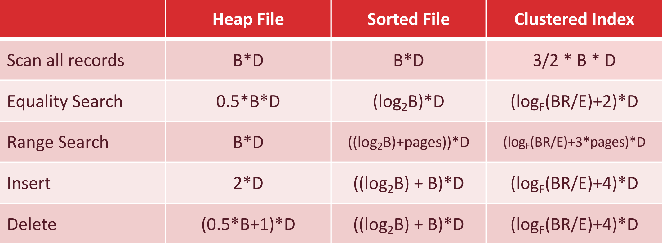
Cost Model for Analysis
- Parameters:
B: Number of data blocks in the fileR: Number of records per blockD: Average time to read/write disk block (We can take out a factor ofDto count the number of I/O instead of estimated time)- (For B+ Tree)
F: Average inner node fanout - (For B+ Tree)
E: Average # data entries per leaf
- Focus: Average case analysis for uniform random workloads for:
- Sequential scan
- Random read
- Random update
- Random insert
- Random delete
- Assumptions: For now, we will ignore:
- Sequential vs Random I/O
- Pre-fetching and cache eviction costs
- Any CPU costs after fetching data into memory
- Reading/writing of header pages for heap files
- Data need to be brought into memory before operated on (and potentially written back to disk afterwards) and both will cost I/O.
- More assumptions:
- Single record insert and delete
- Equality selection – exactly one match
- For Heap Files: Insert always appends to end of file.
- For Sorted Files: Packed means Files compacted after deletions (i.e., no holes); always search according to sorted key.
- Even more assumptions:
- For B+ Tree: assume each page is 2/3 full.
- For B+ Tree: assume using reference as storage method.
Concurrency Control
Recovery
Mechanical Procedures
Size Counting
- Count record size
- Primary key is not nullable.
- Header: Each variable length field needs a 4-Byte pointer to the end of the field in header.
- Header: Each nullable field needs a 1-bit in bitmap in header. Summing them up and round up to the nearest byte for the total size of bitmap.
- Body: For fixed length fields we always allocate the same amount of space even if the field can be NULL, i.e.
topic CHAR[20]will always take 20 bytes. - Body: For variable length fields, if it is nullable it may take up 0 bytes, i.e.
topic VARCHAR[20]will take 0 bytes if it is NULL. If it is not NULL, it may take up a size up to 20 bytes.- This is the only part that makes size of record variable.
- Count records per page
- Exclude all metadata in data page: page header/footer, including bitmap, sibling pointer, free space pointer, slot count etc.
- For page footer layout: Each record needs itself and a slot in the slot directory.
- For fixed length record bitmap layout: Each record needs itself and a bit in the bitmap. Round bitmap to the nearest byte.
- Sometimes we only fill up to a certain percentage of the page.
- Count number of ader pages
- Linked list header page: 1 header page only.
- Page directory header page: number of pages divided by number of entries per page.
- Sometimes need to consider the sibling pointers in header pages when we are counting bytewise.
- Data pages: number of records divided by number of records per page.
I/O Counting
Count heap file I/O (linked list):
- If no implemention specified, ignore header page costs.
- Header pages and sibling pointers both needs maintenance.
- Moving pages between linked lists needs maintenance. Always move to the front of the list to minimize I/O.
- Insert: finding a page in middle of pages with free space might cause more I/O than finding a page at the end of the list. An insertion that causes a page to be full incurs maximum I/O count.
- If record is fixed length, then we can be sure the first non-full page will have enough space.
Count heap file I/O (page directory)
- Full scan: needs to read all header + data pages. (There is no sibling pointer in data pages so we can’t skip header pages.)
- Insert: if primary key is inserted, need a full scan to ensure no duplicate and then + 2 I/Os. If primary key is not inserted, just 2 I/Os.
- Full scan: Do we count in 1 header page?
Count sorted file I/O
- Count as if you can binary search on data pages (without header pages) and you can go to any data page from any page.
Count B+ Tree I/O
- Each node has its own page so reading a node is one I/O.
- Remember to count: reading root, inner, leaf, and actual data page (if implemented with reference).
- Index choice
- If see
ANDcan choose either key on two sides ofAND. - Always choose lower tree with suitable index.
- If see
- If no index, may need to full scan all data pages (ignore trees with irrelevant index). For full scan, ignore tree.
- If data page is changed, index might need changing too which incurs additional write I/O.
- Clustered: to get best-case I/O we can assume everything to be on the same page as much as possible.
- Unclustered: to get worst-case I/O we can assume everything to be on different pages as much as possible.
- One leaf node might need to read many data pages!
- Range query
- Need to count how many leaf nodes are used to encompass the range.
- If alternative 1 storage, data pages themselves are leaf nodes and order number does not apply. Need to check how many records on one data page.
- If alternative 2/3 storage, need to check order number, fill factor.
- Need to count how many leaf nodes are used to encompass the range.
Count Sort I/O: use formula
Count Hash I/O (By example)
- B = 3, N = 8, assuming first partition pass uses a bad hash function, creating a partition A of size 3 and partition B of 5, but the subsequent partition pass uses perfectly uniform hash function.
- Since B = 3, each time we hash pages into two partitions.
- Pass 1:
- Read
8pages. - Write
3 + 5 = 8pages. - In total:
8 + 8 = 16I/Os.
- Read
- Pass 2:
- Partition A only has
3pages so no recursive partitioning needed. - Now for partition B: Read
5pages. - Since hash is uniform now, even partition will have
⌈5/2⌉ = 3pages. - So in total we write
3 + 3 = 6pages. - We can stop for this part, as partition of size 3 will fit in
B = 3. - In total:
5 + 6 = 11I/Os.
- Partition A only has
- Conquer:
- Now, we have
3pages in partition A and6pages in partition B. - Read
3 + 6 = 9pages in total. - Write
3 + 6 = 9pages in total. - In total:
9 + 9 = 18I/Os.
- Now, we have
- Grand total:
16 + 11 + 18 = 45I/Os.
Questions
Questions popped up in my head during the reading:
Can we compress inner nodes in B+ Trees into a single page? (E.g., if the inner node is small enough, we can store it in a single page and use a pointer to the next page to store the rest of the inner node. This is similar to how we store variable length records in pages.)
How to deal with multiple B+ Trees defined over the same table, each wanting its own clustering?
Is it possible to have two clustered indices on separate columns, but you would generally have to store two copies of the data (and keep both up to date).
Special case: if the search key for one index is a subset of the search key for the other (e.g. index 1 on sid, index 2 on (sid, name)), then we can have just one copy (sorted on (sid, name)).How is prefix key compression scalable to insertion?
- Post link: https://reimirno.github.io/2022/10/01/Database-Cheatsheet/
- Copyright Notice: All articles in this blog are licensed under unless otherwise stated.
GitHub Discussions